
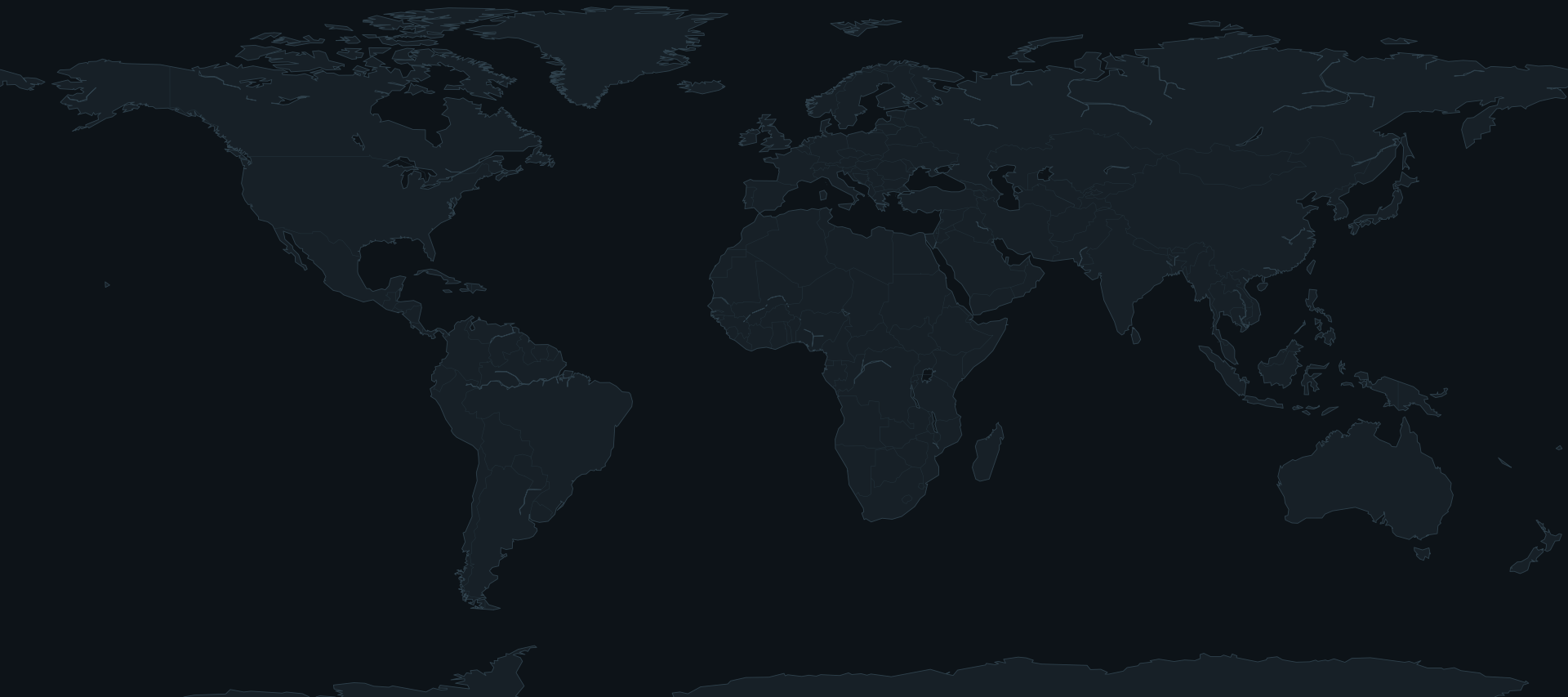
Marker size tracks the composite index; filled markers are inside the window and outlined ones are outside it. To see one field on its own, switch the other domains off in the settings. The projection is equirectangular, so areas away from the equator are stretched: the spread figures are measured on the sphere and are not.
Cambridge
1932Nuclear physics, quantum theory, astronomy, mathematics, economics, philosophy, and the formation of theoretical computing overlapped in a compact town during an exact breakthrough year.
Turing and Chandrasekhar were early in their careers; Keynes divided his time with London.
A flat leading index across a weight sweep means the ordering at the top does not depend on that weight. A step in the eligible count means a filter, not a judgement, decided who was in the room.
There is no single answer, and that is the finding
Ask which place and year had the greatest concentration of consequential people and the question sounds empirical. It is not, until you say what density means. Raw number favours the largest cities. Population adjustment favours the smallest towns. Requiring documented interaction demotes the famous coincidences. Requiring breadth demotes the laboratories. Each of those is a defensible reading, and each elects a different winner from the same sixty-six clusters.
So the weights are not a decoration on top of a result. They are the argument. Move them and watch the top of the table change.
The composite
Six axes on a shared 1 to 5 scale, weighted and renormalised, then discounted for how securely the co-presence is documented:
with , the evidence rating, and the evidence penalty. At the top of the evidence axis the discount is exactly one, so a securely documented cluster is never penalised for being documented.
Three axes that can be computed
Most of what an atlas like this contains is judgement. Three axes are not, because the dataset also carries quantities that are not opinions: a footprint in kilometres, a resident population, and a count of documented pairwise relationships. Proximity holds at the ceiling out to a twenty-minute walk and then decays:
Per-capita intensity is the roster per hundred thousand residents, mapped logarithmically because it spans four orders of magnitude. Interaction is the fraction of possible pairs the record attests, under a square root, because the first documented link in a group of strangers tells you far more than the last one in a group that is already a circle:
Turn on compute the axes in the settings and the composite switches from the judged values to these. The gap between the two versions is the honest measure of how much of the atlas is measurement and how much is assessment.
Two failures worth keeping
The calibration compares each computed axis against the judgement made independently of it. Mean error is 11 per cent across fifteen cases, and two of them miss badly on purpose.
Chicago in 1942 misses by 53 per cent, because the population that mattered was a squash court under a football stand, not a city of three and a half million. Cambridge in 1932 misses by 46 per cent, because the relationship record for fourteen people across four faculties is nowhere near complete, and counting only the famous pairs makes a dense town look like a loose one. Both are cases where the model is wrong in a way that names its own limitation, which is more useful than a table where everything agrees.
Canonical density is not causal density
Vienna in 1913 held Freud, Trotsky, Stalin, and Hitler inside the same city. The relationship graph for that cluster has four nodes and no edges. Jena in November 1799 held seven people inside one house on the Leutragasse, and its graph is nearly complete. A list of names cannot tell those two apart; a graph can. That distinction is why the atlas keeps interaction as a separate axis rather than folding it into co-presence, and why a weighting that ignores it will rank a coincidence above a conversation.
Who is missing
Every roster here is drawn from a canon. Uruk around 3200 BCE probably contained hundreds of consequential people and this atlas can name none of them, so it enters as four anonymous occupational groups and scores accordingly. Timbuktu is suppressed by its surviving archive rather than by its scholarship. Los Alamos and Bell Labs both list eight or ten names in front of thousands of technicians, machinists, and human computers. The co-presence axis measures the visibility of a cluster in the record at least as much as its density.
Model changelog
- proximity: flat at the ceiling out to a 1.5 km walking radius, then 5 * exp(-(f - 1.5) / 14) on the 1 to 5 scale. Decay length anchored on the two extremes of footprint in the corpus and on nothing else.
- per-capita intensity: catalogued people per 100,000 residents, mapped logarithmically as 2.502 + 1.086 * log10(rate). The two constants are anchored on Jena in 1799 and London in 1862, which are therefore excluded from the calibration.
- interaction: graph density over the documented pairwise relationships, mapped as 1 + 4 * sqrt(density). The square root is deliberate: the first links in a group of strangers say more than the last links in a group that is already a circle.
- composite index: weighted sum of six axes on a shared 1 to 5 scale, renormalised, discounted by an evidence factor that reaches exactly one at the top of the certainty axis.
- co-presence field: superposition of Gaussian bumps over a four-segment nonlinear time axis from 3300 BCE to 2026, with local maxima detected on the sampled field and attributed to their top three contributing clusters.
- geography: equirectangular atlas over the same corpus, with duplicate coordinates fanned so five Parises do not render as one marker. Marker area tracks the composite index.
- spread: great-circle distances between the clusters inside the window, reported as the widest pair and the mean pair. This is the complement of footprint, and it answers whether a dense century was one region working or several working independently.
- navigation: the playhead steps between the peak years of eligible clusters rather than the maxima of the smoothed field, because a field maximum is frequently a year containing no cluster at all. Playback, prev, next, random, and keyboard control on top of that.
- filters: footprint cutoff from 200 m to 25 km, temporal window from an exact year to 500 years, an evidence floor, and per-domain toggles. The table falls back to the whole eligible corpus when nothing overlaps the window, and says so.
- presets: six competing definitions of density (balanced, walking distance, one room, who actually talked, raw roster, what got made), each stating the question it asks and the mechanism it exposes rather than the winner it expects.
- calibration: 15 cases as a validation, mean error 11 per cent, worst 53 per cent. Chicago 1942 and Cambridge 1932 are kept in the table precisely because they miss.